Chapter 13 Survival Analysis
https://www.emilyzabor.com/tutorials/survival_analysis_in_r_tutorial.html
over estimating survival if you don’t take into account censoring
library(tidyverse)── Attaching packages ─────────────────────────────────────── tidyverse 1.3.1 ──✔ ggplot2 3.3.5 ✔ purrr 0.3.4
✔ tibble 3.1.4 ✔ dplyr 1.0.7
✔ tidyr 1.1.4 ✔ stringr 1.4.0
✔ readr 2.0.2 ✔ forcats 0.5.1── Conflicts ────────────────────────────────────────── tidyverse_conflicts() ──
✖ dplyr::filter() masks stats::filter()
✖ dplyr::lag() masks stats::lag()cancer <- read_csv("data/survival/veterans_lung_cancer.csv")Rows: 137 Columns: 8── Column specification ────────────────────────────────────────────────────────
Delimiter: ","
chr (3): celltype, prior_therapy, treatment
dbl (4): survival_in_days, age_in_years, karnofsky_score, months_from_diagnosis
lgl (1): status
ℹ Use `spec()` to retrieve the full column specification for this data.
ℹ Specify the column types or set `show_col_types = FALSE` to quiet this message.cancer# A tibble: 137 × 8
status survival_in_days age_in_years celltype karnofsky_score
<lgl> <dbl> <dbl> <chr> <dbl>
1 TRUE 72 69 squamous 60
2 TRUE 411 64 squamous 70
3 TRUE 228 38 squamous 60
4 TRUE 126 63 squamous 60
5 TRUE 118 65 squamous 70
6 TRUE 10 49 squamous 20
7 TRUE 82 69 squamous 40
8 TRUE 110 68 squamous 80
9 TRUE 314 43 squamous 50
10 FALSE 100 70 squamous 70
# … with 127 more rows, and 3 more variables: months_from_diagnosis <dbl>,
# prior_therapy <chr>, treatment <chr>S(t): the survival probability of surviving beyond time,tgivin they have survived until now.
library(survival)
Attaching package: 'survival'The following object is masked _by_ '.GlobalEnv':
cancerThe survival object uses the Surv function.
The + denotes a censored subject.
Surv(cancer$survival_in_days, cancer$status) [1] 72 411 228 126 118 10 82 110 314 100+ 42 8 144 25+ 11
[16] 30 384 4 54 13 123+ 97+ 153 59 117 16 151 22 56 21
[31] 18 139 20 31 52 287 18 51 122 27 54 7 63 392 10
[46] 8 92 35 117 132 12 162 3 95 177 162 216 553 278 12
[61] 260 200 156 182+ 143 105 103 250 100 999 112 87+ 231+ 242 991
[76] 111 1 587 389 33 25 357 467 201 1 30 44 283 15 25
[91] 103+ 21 13 87 2 20 7 24 99 8 99 61 25 95 80
[106] 51 29 24 18 83+ 31 51 90 52 73 8 36 48 7 140
[121] 186 84 19 45 80 52 164 19 53 15 43 340 133 111 231
[136] 378 49 Create the survival curve
sf1 <- survfit(Surv(cancer$survival_in_days, cancer$status) ~ 1, data = cancer)
sf1
Call: survfit(formula = Surv(cancer$survival_in_days, cancer$status) ~
1, data = cancer)
n events median 0.95LCL 0.95UCL
[1,] 137 128 80 52 105names(sf1) [1] "n" "time" "n.risk" "n.event" "n.censor" "surv"
[7] "std.err" "cumhaz" "std.chaz" "type" "logse" "conf.int"
[13] "conf.type" "lower" "upper" "call" time: time inverval start and endpointssurv: sruvival prbability at eachtime
library(survminer)Loading required package: ggpubr
Attaching package: 'survminer'The following object is masked from 'package:survival':
myelomaggsurvplot(
fit = sf1,
xlab = "Days",
ylab = "Overall survival probability")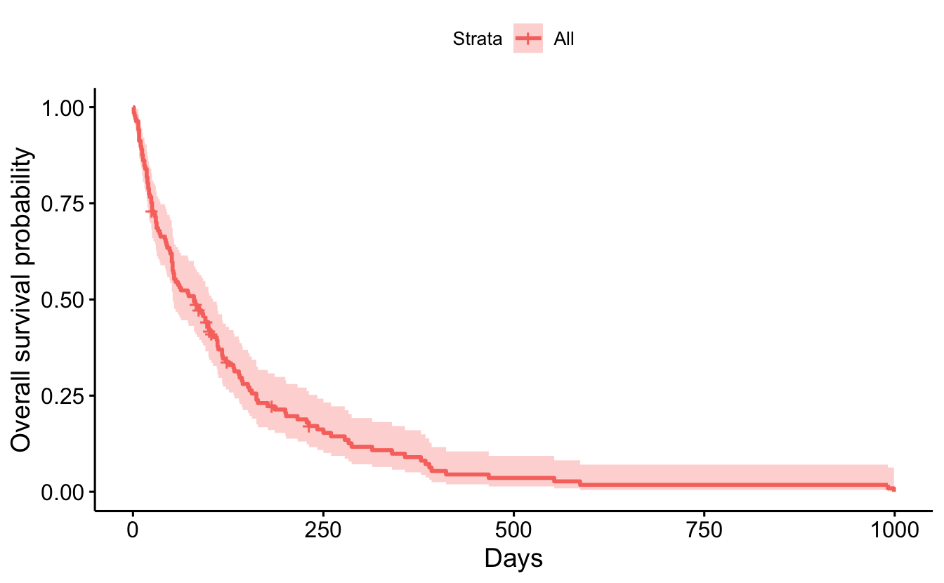
summary(sf1, times = 365.25)Call: survfit(formula = Surv(cancer$survival_in_days, cancer$status) ~
1, data = cancer)
time n.risk n.event survival std.err lower 95% CI upper 95% CI
365 10 118 0.09 0.0265 0.0506 0.1613.1 Between Groups
sf2 <- survfit(Surv(survival_in_days, status) ~ treatment, data = cancer)
summary(sf2, times = 365.25)
Call: survfit(formula = Surv(survival_in_days, status) ~ treatment,
data = cancer)
treatment=standard
time n.risk n.event survival std.err lower 95% CI
365.2500 4.0000 60.0000 0.0708 0.0336 0.0279
upper 95% CI
0.1795
treatment=test
time n.risk n.event survival std.err lower 95% CI
365.2500 6.0000 58.0000 0.1098 0.0407 0.0530
upper 95% CI
0.2272 ggsurvplot(
fit = sf2,
data = cancer,
xlab = "Days",
ylab = "Overall survival probability",
risk.table = TRUE)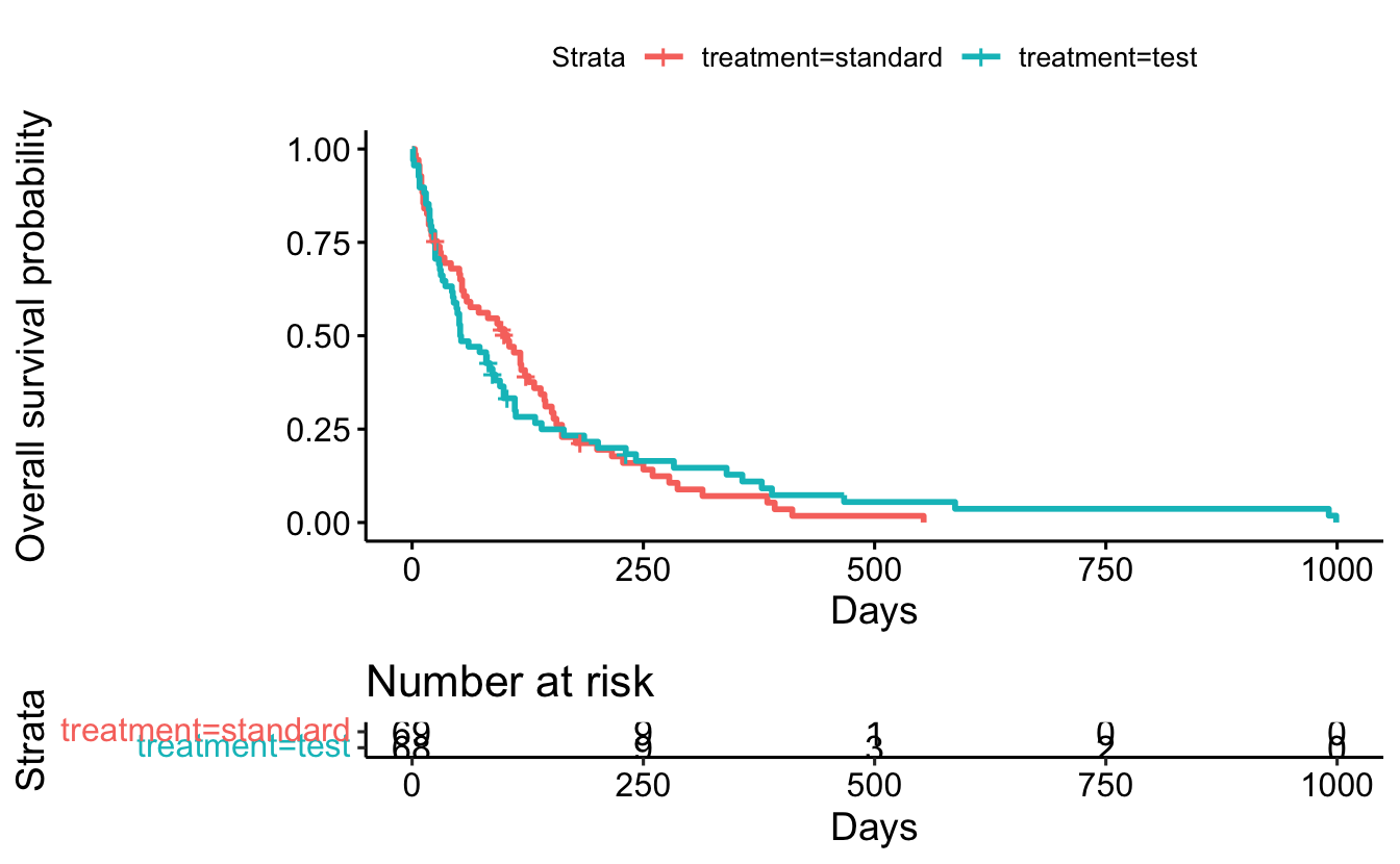
13.2 Multiple variables
sf3 <- survfit(Surv(survival_in_days, status) ~ prior_therapy, data = cancer)ggsurvplot(
fit = sf3,
data = cancer,
risk.table = TRUE,
conf.int = TRUE)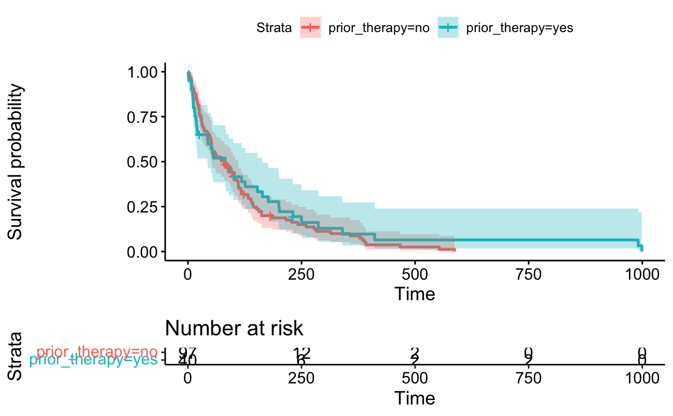
sf4 <- survfit(Surv(survival_in_days, status) ~ treatment + prior_therapy, data = cancer)

summary(sf4, times = 365.25)
Call: survfit(formula = Surv(survival_in_days, status) ~ treatment +
prior_therapy, data = cancer)
treatment=standard, prior_therapy=no
time n.risk n.event survival std.err lower 95% CI
365.2500 3.0000 41.0000 0.0807 0.0436 0.0280
upper 95% CI
0.2326
treatment=standard, prior_therapy=yes
time n.risk n.event survival std.err lower 95% CI
3.65e+02 1.00e+00 1.90e+01 5.16e-02 5.02e-02 7.67e-03
upper 95% CI
3.47e-01
treatment=test, prior_therapy=no
time n.risk n.event survival std.err lower 95% CI
365.2500 4.0000 43.0000 0.0916 0.0432 0.0363
upper 95% CI
0.2310
treatment=test, prior_therapy=yes
time n.risk n.event survival std.err lower 95% CI
365.2500 2.0000 15.0000 0.1604 0.0944 0.0506
upper 95% CI
0.5082 ggsurvplot(
fit = sf4,
data = cancer)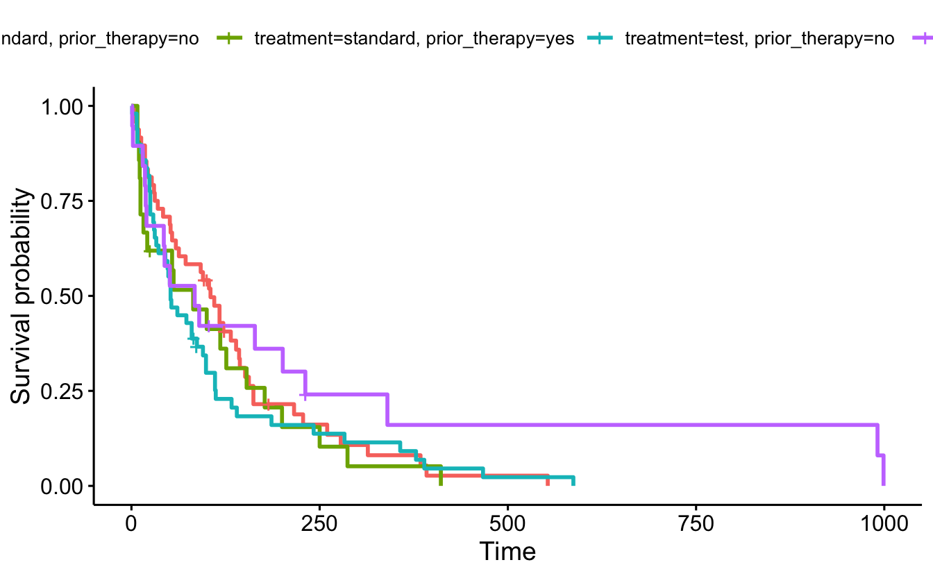
13.3 Cox Regression
h(t): hazard, the instantaneous rate at which events occur
coxph(Surv(survival_in_days, status) ~ treatment + prior_therapy, data = cancer)Call:
coxph(formula = Surv(survival_in_days, status) ~ treatment +
prior_therapy, data = cancer)
coef exp(coef) se(coef) z p
treatmenttest 0.02608 1.02643 0.18099 0.144 0.885
prior_therapyyes -0.14474 0.86525 0.20091 -0.720 0.471
Likelihood ratio test=0.54 on 2 df, p=0.7636
n= 137, number of events= 128 13.3.1 Hazard Ratio
library(broom)coxph(Surv(survival_in_days, status) ~ treatment + prior_therapy, data = cancer) %>%
tidy() %>%
mutate(hr = exp(estimate))# A tibble: 2 × 6
term estimate std.error statistic p.value hr
<chr> <dbl> <dbl> <dbl> <dbl> <dbl>
1 treatmenttest 0.0261 0.181 0.144 0.885 1.03
2 prior_therapyyes -0.145 0.201 -0.720 0.471 0.865Taken from Emily’s page (for now) https://www.emilyzabor.com/tutorials/survival_analysis_in_r_tutorial.html
The quantity of interest from a Cox regression model is a hazard ratio (HR). The HR represents the ratio of hazards between two groups at any particular point in time.

The HR is interpreted as the instantaneous rate of occurrence of the event of interest in those who are still at risk for the event. It is not a risk, though it is commonly interpreted as such.

If you have a regression parameter β
(from column estimate in our coxph) then HR = exp(β)

.

A HR < 1 indicates reduced hazard of death whereas a HR > 1 indicates an increased hazard of death.

our treatmenttest = 1.03 implies that around 1 times as many test are dying as standard, at any given time.
out prior_therapyyes = 0.865 implies that around 0.865 times as many yesprior are dying as noprior, at any given time.
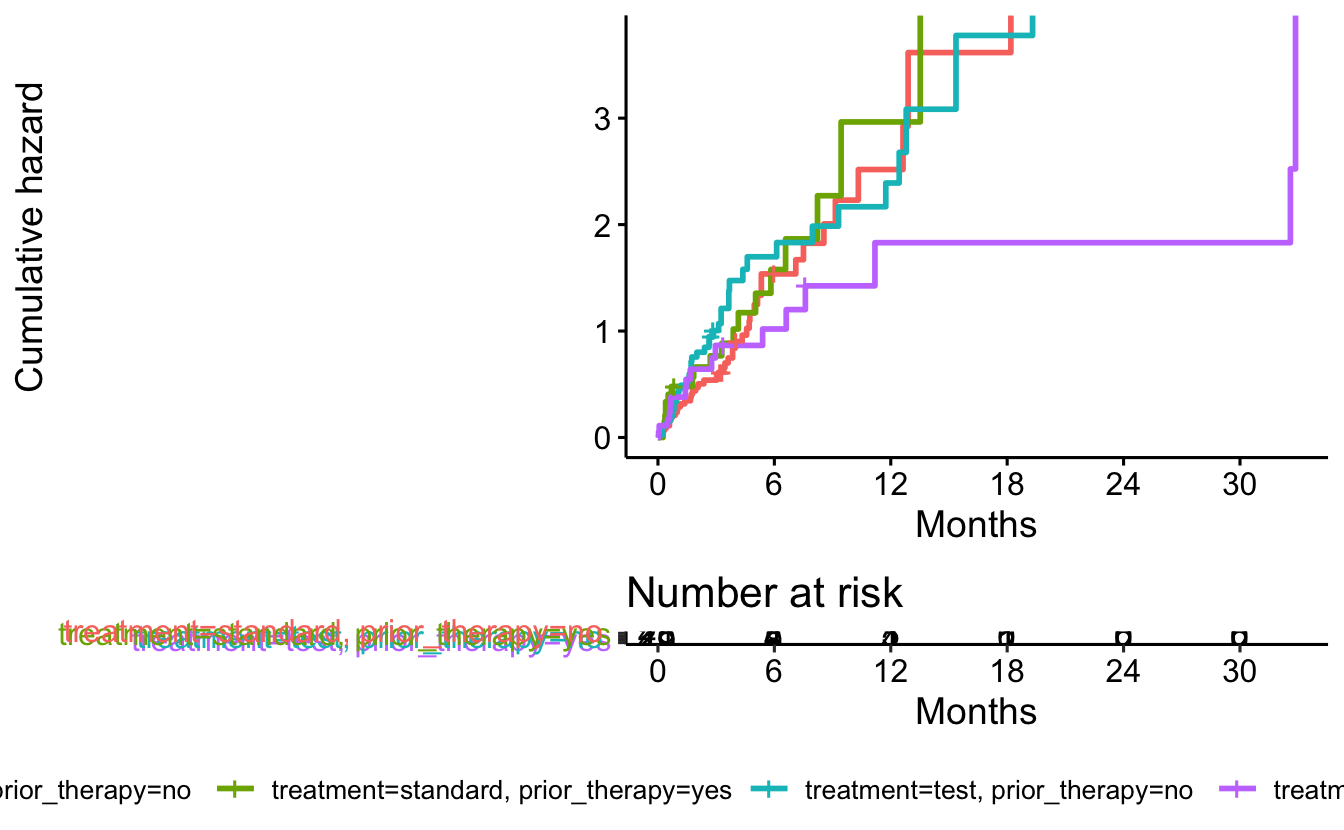
fit <- survfit(Surv(survival_in_days, status) ~ treatment + prior_therapy, data = cancer)ggsurvplot(data = cancer,
fit = fit,
risk.table = TRUE,
fun = "cumhaz",
legend = "bottom",
legend.title = "",
xlab = "Months",
xscale = 30.4,
break.x.by = 182.4
)