Chapter 14 Machine Learning (tidymodels)
https://conf20-intro-ml.netlify.app/
14.1 Logistic Regression
library(tidyverse)── Attaching packages ─────────────────────────────────────── tidyverse 1.3.1 ──✔ ggplot2 3.3.5 ✔ purrr 0.3.4
✔ tibble 3.1.4 ✔ dplyr 1.0.7
✔ tidyr 1.1.4 ✔ stringr 1.4.0
✔ readr 2.0.2 ✔ forcats 0.5.1── Conflicts ────────────────────────────────────────── tidyverse_conflicts() ──
✖ dplyr::filter() masks stats::filter()
✖ dplyr::lag() masks stats::lag()library(medicaldata)
library(broom)blood <- blood_storageblood$Recurrence <- as.factor(blood$Recurrence)
blood$RBC.Age.Group <- as.factor(blood$RBC.Age.Group)14.1.1 glm: Model 1
mod <- glm(Recurrence ~ RBC.Age.Group, data = blood, family = "binomial")
summary(mod)
Call:
glm(formula = Recurrence ~ RBC.Age.Group, family = "binomial",
    data = blood)

Deviance Residuals:
    Min       1Q   Median       3Q      Max
-0.6285  -0.6285  -0.6069  -0.6006   1.8982

Coefficients:
               Estimate Std. Error z value Pr(>|z|)
(Intercept)    -1.52147    0.25323  -6.008 1.88e-09 ***
RBC.Age.Group2 -0.09966    0.36685  -0.272    0.786
RBC.Age.Group3 -0.07680    0.36183  -0.212    0.832
---
Signif. codes:  0 '***' 0.001 '**' 0.01 '*' 0.05 '.' 0.1 ' ' 1

(Dispersion parameter for binomial family taken to be 1)

    Null deviance: 289.01  on 315  degrees of freedom
Residual deviance: 288.92  on 313  degrees of freedom
AIC: 294.92

Number of Fisher Scoring iterations: 4
mod %>%
broom::tidy() %>%
mutate(or = exp(estimate))# A tibble: 3 × 6
term estimate std.error statistic p.value or
<chr> <dbl> <dbl> <dbl> <dbl> <dbl>
1 (Intercept) -1.52 0.253 -6.01 0.00000000188 0.218
2 RBC.Age.Group2 -0.0997 0.367 -0.272 0.786 0.905
3 RBC.Age.Group3 -0.0768 0.362 -0.212 0.832 0.92614.1.2 glm: Model 2
Recurrence ~ Age + PVol + PreopPSA + as.factor(TVol) + as.factor(RBC.Age.Group)Recurrence ~ Age + PVol + PreopPSA + as.factor(TVol) + as.factor(RBC.Age.Group)mod <- glm(Recurrence ~ Age + PVol + PreopPSA + as.factor(TVol) + as.factor(RBC.Age.Group), data = blood, family = "binomial")
summary(mod)
Call:
glm(formula = Recurrence ~ Age + PVol + PreopPSA + as.factor(TVol) +
    as.factor(RBC.Age.Group), family = "binomial", data = blood)

Deviance Residuals:
    Min       1Q   Median       3Q      Max
-1.4637  -0.5829  -0.4627  -0.1675   2.7398

Coefficients:
                            Estimate Std. Error z value Pr(>|z|)
(Intercept)               -6.139e+00  1.840e+00  -3.336 0.000851 ***
Age                        2.672e-02  2.449e-02   1.091 0.275156
PVol                       4.581e-05  6.528e-03   0.007 0.994401
PreopPSA                   5.969e-02  2.448e-02   2.438 0.014784 *
as.factor(TVol)2           2.071e+00  1.063e+00   1.947 0.051543 .
as.factor(TVol)3           3.128e+00  1.068e+00   2.930 0.003391 **
as.factor(RBC.Age.Group)2 -2.263e-01  4.248e-01  -0.533 0.594152
as.factor(RBC.Age.Group)3  1.144e-01  4.011e-01   0.285 0.775461
---
Signif. codes:  0 '***' 0.001 '**' 0.01 '*' 0.05 '.' 0.1 ' ' 1

(Dispersion parameter for binomial family taken to be 1)

    Null deviance: 267.09  on 299  degrees of freedom
Residual deviance: 228.72  on 292  degrees of freedom
  (16 observations deleted due to missingness)
AIC: 244.72

Number of Fisher Scoring iterations: 6
mod %>%
broom::tidy() %>%
mutate(or = exp(estimate))# A tibble: 8 × 6
term estimate std.error statistic p.value or
<chr> <dbl> <dbl> <dbl> <dbl> <dbl>
1 (Intercept) -6.14 1.84 -3.34 0.000851 0.00216
2 Age 0.0267 0.0245 1.09 0.275 1.03
3 PVol 0.0000458 0.00653 0.00702 0.994 1.00
4 PreopPSA 0.0597 0.0245 2.44 0.0148 1.06
5 as.factor(TVol)2 2.07 1.06 1.95 0.0515 7.93
6 as.factor(TVol)3 3.13 1.07 2.93 0.00339 22.8
7 as.factor(RBC.Age.Group)2 -0.226 0.425 -0.533 0.594 0.797
8 as.factor(RBC.Age.Group)3 0.114 0.401 0.285 0.775 1.12 14.2 Tidymodels
library(tidymodels)Registered S3 method overwritten by 'tune':
method from
required_pkgs.model_spec parsnip── Attaching packages ────────────────────────────────────── tidymodels 0.1.3 ──✔ dials 0.0.10 ✔ rsample 0.1.0
✔ infer 1.0.0 ✔ tune 0.1.6
✔ modeldata 0.1.1 ✔ workflows 0.2.3
✔ parsnip 0.1.7 ✔ workflowsets 0.1.0
✔ recipes 0.1.17 ✔ yardstick 0.0.8 ── Conflicts ───────────────────────────────────────── tidymodels_conflicts() ──
✖ scales::discard() masks purrr::discard()
✖ dplyr::filter() masks stats::filter()
✖ recipes::fixed() masks stringr::fixed()
✖ dplyr::lag() masks stats::lag()
✖ yardstick::spec() masks readr::spec()
✖ recipes::step() masks stats::step()
• Use tidymodels_prefer() to resolve common conflicts.model <- logistic_reg()model %>% translate()Logistic Regression Model Specification (classification)
Computational engine: glm
Model fit template:
stats::glm(formula = missing_arg(), data = missing_arg(), weights = missing_arg(),
family = stats::binomial)model_fit <- model %>%
fit(Recurrence ~ Age + PVol + PreopPSA + as.factor(TVol) + as.factor(RBC.Age.Group), data = blood)model_fit %>%
broom::tidy() %>%
mutate(or = exp(estimate))# A tibble: 8 × 6
term estimate std.error statistic p.value or
<chr> <dbl> <dbl> <dbl> <dbl> <dbl>
1 (Intercept) -6.14 1.84 -3.34 0.000851 0.00216
2 Age 0.0267 0.0245 1.09 0.275 1.03
3 PVol 0.0000458 0.00653 0.00702 0.994 1.00
4 PreopPSA 0.0597 0.0245 2.44 0.0148 1.06
5 as.factor(TVol)2 2.07 1.06 1.95 0.0515 7.93
6 as.factor(TVol)3 3.13 1.07 2.93 0.00339 22.8
7 as.factor(RBC.Age.Group)2 -0.226 0.425 -0.533 0.594 0.797
8 as.factor(RBC.Age.Group)3 0.114 0.401 0.285 0.775 1.12 14.2.1 Make a prediction
There are many problems with this. Also class imbalance is coming into play.
blood_sample <- blood %>% dplyr::sample_n(10)

blood_sample
RBC.Age.Group Median.RBC.Age Age AA FamHx PVol TVol T.Stage bGS BN+
1 2 15 62.4 1 0 74.0 1 1 1 0
2 1 10 55.9 0 0 20.9 3 1 2 0
3 3 25 71.8 0 1 99.8 2 1 1 0
4 2 15 68.3 0 0 41.7 2 1 2 0
5 3 25 56.0 0 1 68.0 1 1 1 0
6 2 15 57.9 0 0 63.4 2 1 1 0
7 3 25 59.9 0 1 54.1 3 1 1 0
8 2 15 64.5 0 0 60.0 2 1 1 0
9 3 25 66.1 0 0 32.2 2 1 3 0
10 2 15 57.9 0 1 24.0 2 NA 1 0
OrganConfined PreopPSA PreopTherapy Units sGS AnyAdjTherapy AdjRadTherapy
1 1 6.27 0 3 2 0 0
2 0 5.10 1 2 1 0 0
3 1 5.40 0 1 2 0 0
4 0 6.75 0 3 3 0 0
5 1 8.30 0 5 2 0 0
6 1 4.89 0 4 3 0 0
7 1 6.80 0 1 3 0 0
8 1 1.80 0 4 2 0 0
9 1 7.50 0 2 4 0 0
10 1 5.00 0 2 3 0 0
Recurrence Censor TimeToRecurrence
1 0 1 13.90
2 1 0 24.60
3 0 1 93.80
4 0 1 4.73
5 0 1 65.00
6 0 1 22.26
7 0 1 24.87
8 0 1 103.60
9 1 0 2.60
10 0 1 7.49predict(model_fit, blood_sample)# A tibble: 10 × 1
.pred_class
<fct>
1 0
2 0
3 0
4 0
5 0
6 0
7 0
8 0
9 0
10 0 14.3 Train Test Split
set.seed(42)
blood_split <- initial_split(blood, prop = 0.80, strata = Recurrence)
blood_train <- training(blood_split)
blood_test  <-  testing(blood_split)
model <- logistic_reg()
model_fit <- model %>%
fit(Recurrence ~ Age + PVol + PreopPSA + as.factor(TVol) + as.factor(RBC.Age.Group),
data = blood_train)
summary(model_fit$fit)
Call:
stats::glm(formula = Recurrence ~ Age + PVol + PreopPSA + as.factor(TVol) +
    as.factor(RBC.Age.Group), family = stats::binomial, data = data)

Deviance Residuals:
    Min       1Q   Median       3Q      Max
-1.5393  -0.6221  -0.4638  -0.2001   2.5484

Coefficients:
                           Estimate Std. Error z value Pr(>|z|)
(Intercept)               -7.524502   2.080897  -3.616 0.000299 ***
Age                        0.060840   0.029379   2.071 0.038371 *
PVol                      -0.005528   0.007349  -0.752 0.451959
PreopPSA                   0.063272   0.027640   2.289 0.022069 *
as.factor(TVol)2           1.714091   1.061132   1.615 0.106237
as.factor(TVol)3           2.633132   1.069533   2.462 0.013819 *
as.factor(RBC.Age.Group)2 -0.270055   0.465377  -0.580 0.561717
as.factor(RBC.Age.Group)3  0.082405   0.443813   0.186 0.852700
---
Signif. codes:  0 '***' 0.001 '**' 0.01 '*' 0.05 '.' 0.1 ' ' 1

(Dispersion parameter for binomial family taken to be 1)

    Null deviance: 219.46  on 239  degrees of freedom
Residual deviance: 189.46  on 232  degrees of freedom
  (12 observations deleted due to missingness)
AIC: 205.46

Number of Fisher Scoring iterations: 6
model_fit %>%
broom::tidy() %>%
mutate(or = exp(estimate))# A tibble: 8 × 6
term estimate std.error statistic p.value or
<chr> <dbl> <dbl> <dbl> <dbl> <dbl>
1 (Intercept) -7.52 2.08 -3.62 0.000299 0.000540
2 Age 0.0608 0.0294 2.07 0.0384 1.06
3 PVol -0.00553 0.00735 -0.752 0.452 0.994
4 PreopPSA 0.0633 0.0276 2.29 0.0221 1.07
5 as.factor(TVol)2 1.71 1.06 1.62 0.106 5.55
6 as.factor(TVol)3 2.63 1.07 2.46 0.0138 13.9
7 as.factor(RBC.Age.Group)2 -0.270 0.465 -0.580 0.562 0.763
8 as.factor(RBC.Age.Group)3 0.0824 0.444 0.186 0.853 1.09 model_predict <- predict(model_fit, blood_test)model_predict# A tibble: 64 × 1
.pred_class
<fct>
1 0
2 1
3 0
4 0
5 0
6 0
7 0
8 0
9 <NA>
10 0
# … with 54 more rows14.4 Get class predictions and probabilties
model_predict %>%
  count(`.pred_class`)
# A tibble: 3 × 2
.pred_class n
<fct> <int>
1 0 59
2 1 1
3 <NA> 4model_predict# A tibble: 64 × 1
.pred_class
<fct>
1 0
2 1
3 0
4 0
5 0
6 0
7 0
8 0
9 <NA>
10 0
# … with 54 more rowsmodel_predict_class <- predict(model_fit, blood_test)
model_predict_class# A tibble: 64 × 1
.pred_class
<fct>
1 0
2 1
3 0
4 0
5 0
6 0
7 0
8 0
9 <NA>
10 0
# … with 54 more rowsmodel_predict_prop <- predict(model_fit, blood_test, type = "prob")
model_predict_prop# A tibble: 64 × 2
.pred_0 .pred_1
<dbl> <dbl>
1 0.892 0.108
2 0.408 0.592
3 0.739 0.261
4 0.869 0.131
5 0.969 0.0313
6 0.994 0.00638
7 0.789 0.211
8 0.880 0.120
9 NA NA
10 0.981 0.0188
# … with 54 more rowsblood_results <- bind_cols(model_predict_class, model_predict_prop, blood_test %>% select(Recurrence)) %>%
tidyr::drop_na()
blood_results# A tibble: 60 × 4
.pred_class .pred_0 .pred_1 Recurrence
<fct> <dbl> <dbl> <fct>
1 0 0.892 0.108 0
2 1 0.408 0.592 0
3 0 0.739 0.261 0
4 0 0.869 0.131 0
5 0 0.969 0.0313 0
6 0 0.994 0.00638 0
7 0 0.789 0.211 0
8 0 0.880 0.120 0
9 0 0.981 0.0188 0
10 0 0.888 0.112 0
# … with 50 more rows14.5 Model Metrics and Evaluation
conf_mat(blood_results, truth = Recurrence, estimate = .pred_class) Truth
Prediction 0 1
0 51 8
1 1 0accuracy(blood_results, truth = Recurrence, estimate = .pred_class)# A tibble: 1 × 3
.metric .estimator .estimate
<chr> <chr> <dbl>
1 accuracy binary 0.85sens(blood_results, truth = Recurrence, estimate = .pred_class)# A tibble: 1 × 3
.metric .estimator .estimate
<chr> <chr> <dbl>
1 sens binary 0.981specificity(blood_results, truth = Recurrence, estimate = .pred_class)# A tibble: 1 × 3
.metric .estimator .estimate
<chr> <chr> <dbl>
1 spec binary 0precision(blood_results, truth = Recurrence, estimate = .pred_class)# A tibble: 1 × 3
.metric .estimator .estimate
<chr> <chr> <dbl>
1 precision binary 0.864recall(blood_results, truth = Recurrence, estimate = .pred_class)# A tibble: 1 × 3
.metric .estimator .estimate
<chr> <chr> <dbl>
1 recall binary 0.981my_metrics <- metric_set(sensitivity, specificity)
my_metrics(blood_results, truth = Recurrence, estimate = .pred_class)# A tibble: 2 × 3
.metric .estimator .estimate
<chr> <chr> <dbl>
1 sens binary 0.981
2 spec binary 0 roc_auc(blood_results, truth = Recurrence, estimate = .pred_1)# A tibble: 1 × 3
.metric .estimator .estimate
<chr> <chr> <dbl>
1 roc_auc binary 0.243roc_curve(blood_results, truth = Recurrence, estimate = .pred_0) %>%
autoplot()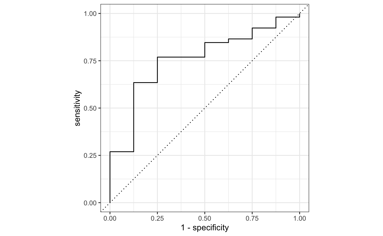
14.6 Feature Engineering
library(themis)Registered S3 methods overwritten by 'themis':
method from
bake.step_downsample recipes
bake.step_upsample recipes
prep.step_downsample recipes
prep.step_upsample recipes
tidy.step_downsample recipes
tidy.step_upsample recipes
tunable.step_downsample recipes
tunable.step_upsample recipes
Attaching package: 'themis'The following objects are masked from 'package:recipes':
step_downsample, step_upsampleblood <- blood_storageblood$Recurrence <- as.factor(blood$Recurrence)blood_split <- initial_split(blood, prop = 0.80, strata = Recurrence)
blood_train <- training(blood_split)
blood_test <- testing(blood_split)simple_blood <-
recipe(Recurrence ~ Age + PVol + PreopPSA + TVol + RBC.Age.Group,
data = blood_train) %>%
step_mutate(TVol = as.factor(TVol),
RBC.Age.Group = as.factor(RBC.Age.Group),
role = "predictor"
) %>%
step_dummy(all_nominal_predictors()) %>%
step_zv(all_predictors()) %>%
themis::step_downsample(Recurrence)
simple_bloodRecipe
Inputs:
role #variables
outcome 1
predictor 5
Operations:
Variable mutation
Dummy variables from all_nominal_predictors()
Zero variance filter on all_predictors()
Down-sampling based on Recurrencelogistic_model <- logistic_reg() %>%
set_engine("glm")
logistic_wflow2 <-
workflow() %>%
add_model(logistic_model) %>%
add_recipe(simple_blood)
logistic_fit <- fit(logistic_wflow2, blood_train)Warning: There are new levels in a factor: NAlogistic_fit %>% extract_recipe(estimated = TRUE)Recipe
Inputs:
role #variables
outcome 1
predictor 5
Training data contained 252 data points and 14 incomplete rows.
Operations:
Variable mutation [trained]
Dummy variables from TVol, RBC.Age.Group [trained]
Zero variance filter removed no terms [trained]
Down-sampling based on Recurrence [trained]logistic_fit %>% tidy() %>% mutate(or = exp(estimate))# A tibble: 8 × 6
term estimate std.error statistic p.value or
<chr> <dbl> <dbl> <dbl> <dbl> <dbl>
1 (Intercept) -22.8 1776. -0.0129 0.990 1.22e-10
2 Age 0.0440 0.0352 1.25 0.211 1.04e+ 0
3 PVol 0.00131 0.0158 0.0828 0.934 1.00e+ 0
4 PreopPSA 0.0947 0.0583 1.62 0.104 1.10e+ 0
5 TVol_X2 19.0 1776. 0.0107 0.991 1.86e+ 8
6 TVol_X3 19.6 1776. 0.0110 0.991 3.23e+ 8
7 RBC.Age.Group_X2 0.347 0.691 0.503 0.615 1.42e+ 0
8 RBC.Age.Group_X3 0.261 0.665 0.392 0.695 1.30e+ 0predict(logistic_fit, blood_test)# A tibble: 64 × 1
.pred_class
<fct>
1 0
2 1
3 0
4 0
5 0
6 0
7 0
8 1
9 0
10 0
# … with 54 more rows