Chapter 6 Clean Data (Tidy)

Figure 0.2: “Data Cowboy” by Allison Horst.
6.1 Introduction
Now that we have seen how to import a dataset as a dataframe object, we can start the process of “cleaning” it. We saw in the “Spreadsheets” Chapter (2) that data could come in different formats and “shapes” that serve different purposes. Our Goal now is to start the process of making our dataset “clean” by making it more amenable to different visualization and modeling methods. Cleaning, processing, wrangling, tidying, etc are all synonyms you may have heard being used for this process (others include screaming, cursing, and walking away).
This chapter is one of the most important concepts in data processing. It creates a standardized way to talk about a “clean” dataset and structures how you can process your data. It also serves as a great common ground to move between different programming languages, since the data manipulation steps are common throughout different languages, only the actual programming syntax will change.
6.2 What is tidy data?
When we want to “clean” data, there needs to be some standard way to describe what we mean and some goal to work towards when we are cleaning our dataset. Hadley Wickham’s 2014 “Tidy Data” paper in the Journal of Statistical Software gives us a formal definition we can use to describe the “shape” of our data. We will use examples from the paper to define “tidy data”.
Below is a duplicate of “Tidy Data’s” Table 1. It shows an example dataset where each row represents a person and columns for some imaginary experiment’s treatment values.
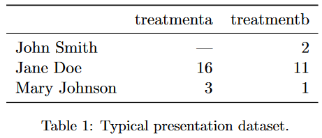
This is a space efficient representation of our data. It allows the reader to quickly glance the data values and perform comparisons in their heads.
We can also transpose the values of our dataset so the rows and columns are interchanged.
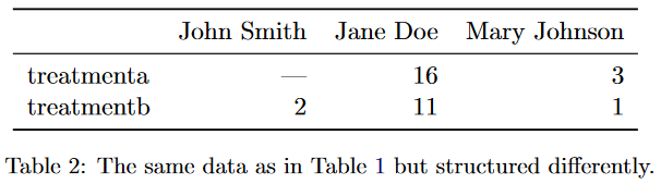
Other than making the dataset “wider”, we can still do the same set of quick comparisons in this data representation.
These two “shapes” of the same dataset are good for presentations when data needs to be quickly interpreted by a user.
However, remember the group_by function we first used in Chapter 5.1,
we are unable to perform those aggregate summary statistics in the way our dataset is formatted.
If we organize the data into another shape:
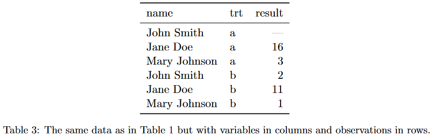
We can see it makes doing treatment comparisons more difficult as a reader. However, we can now answer the question of “what is the average value for each treatment?” and from a statistical analysis point of view, we can now answer the question of “how does treatment affect the result?”. This last example is the “tidy” or “clean” form of our example dataset.
So what aspects of the last table example make it tidy? The “Tidy Data” paper defines “tidy data” as having 3 features
- Each variable forms a column
- Each observation forms a row
- Each cell is a single measurement
If we compare the “tidy data” definition, we can see how the first 2 table examples violate the “tidy data” definition. We want a “variable” for person, treatment, and value, not each column containing a single treatment’s value or a single person’s value. The unit of interest our dataset stores is a person’s treatment value, so each row should represent a person.
 blog [*Tidy Data for reproducibility, efficiency, and collaboration*](https://www.openscapes.org/blog/2020/10/12/tidy-data/) by Julia Lowndes and Allison Horst](https://github.com/allisonhorst/stats-illustrations/raw/master/rstats-artwork/tidydata_1.jpg)
Figure 0.6: “Tidy data is a standard way of mapping the meaning of a dataset to its structure” - Hadley Wickham. In tidy data: each variable forms a column, each observation forms a row, and each cell is a single measurement. Wickham, H (2014). Tidy Data. Journal of Statistical Software 59 (10). DOT: 10.18637/jss.v059.i10. Illustrations from the Openscapes blog Tidy Data for reproducibility, efficiency, and collaboration by Julia Lowndes and Allison Horst
This now gives us the framework to process data so we can begin working with disparate data sets.

Now that data can be consistently formatted, when we describe a dataset as being “tidy”, we know what that means. This also makes creating tools and analysis pipelines easier since the shape of our data will be consistent.

Once you have a tidy dataset, you can easily transform it back to a more presentation friendly view.
6.3 Common data problems
We’ve discussed what makes data “tidy”, but what about actually doing it? Most of the “messy” data sets we see in the world can actually be described as having the same “problems”.
- Column headers are values, not variable names
- Multiple variables stored in one column
- Variables are stored in both rows and columns
We will discuss each point in more detail in the following sections.
 blog [*Tidy Data for reproducibility, efficiency, and collaboration*](https://www.openscapes.org/blog/2020/10/12/tidy-data/) by Julia Lowndes and Allison Horst](https://github.com/allisonhorst/stats-illustrations/raw/master/rstats-artwork/tidydata_2.jpg)
Figure 0.9: “The standard structure of tidy means that ’tidy datasets are all alike … but every messy dataset is messy in its own way.” - Hadley Wickham. Tidy data sets saying “Our columns are variables and our rows are observations”, messy data sets saying “my columns are values and my rows are variables; I have variables in columns and in rows; I have multiple variables in a single columns; I don’t even know what my deal is”. Illustrations from the Openscapes blog Tidy Data for reproducibility, efficiency, and collaboration by Julia Lowndes and Allison Horst
6.4 Column headers are values, not variable names
This dataset from the Pew Research Center explores the relationship between income and religion in the US. It shows the religion and frequency for a particular income bracket.
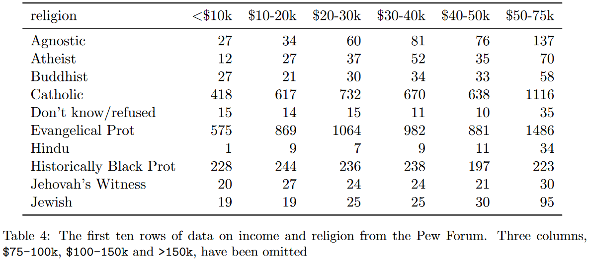
Figure 0.10: Table 4 from the “Tidy Data” paper.
We listed 3 variables the table depicts, but those 3 variables are not the variables (i.e., columns) of the dataset. The values of the “income” variable are actually the columns of our dataset. This is the “column headers are values, not variable names” problem with our current dataset. If we wanted to make it tidy, such that we had 3 columns (religion, income, and frequency), the data set would look as follows:
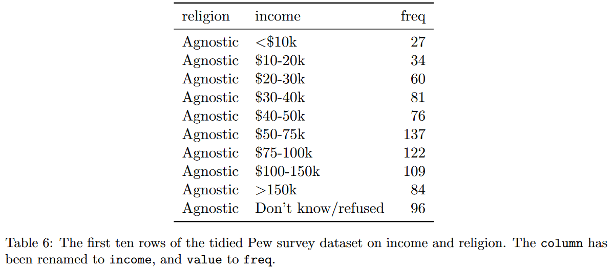
Figure 0.11: Table 6 from the “Tidy Data” paper.
The first table is sometimes called the wide format since it has more columns and wider to print on the screen, and the tidy version of the data set example is sometimes called the long format since it has more rows and is longer to print on the screen.
Let’s go through an example by loading up the tidyverse library and our dataset.
Note that the code below has suppressed the message output from loading the library and reading in the dataset.
R
library(tidyverse)
tumor <- read_csv("./data/tumorgrowth_long.csv")
Python
import pandas as pd

tumor = pd.read_csv("./data/tumorgrowth_long.csv")
This dataset comes from the medicaldata R package,
curated by Dr. Peter Higgins, M.D. in the
IBD Research Group at the University of Michigan Medical School.
The dataset we loaded is a modified version of the “tumorgrowth” dataset in the medicaldata package.
It shows the treatment group for a particular sample and its size (\(mm^3\)) over time (days).
Cells from a human glioma cell line were implanted in the flank of n=37 nude mice and a subcutaneous tumor (xenograft) was allowed to grow. When a tumor grew to around 40-60mm^3, the animal was assigned to one of 4 experimenal groups… The main outcome in xenograft experiments is the size (volume) of the tumor over time.
You can read more about the dataset and study in the codebook for “Mixed-Effects Modeling of Tumor Growth in Animal Xenograft Experiments”
R
tumor# A tibble: 37 × 32
Group Grp ID `0` `1` `2` `3` `4` `5` `6` `7` `8` `9`
<dbl> <chr> <dbl> <dbl> <dbl> <dbl> <dbl> <dbl> <dbl> <dbl> <dbl> <dbl> <dbl>
1 1 1.CTR 101 41.8 NA NA 85 114 162. 178. 325 NA NA
2 1 1.CTR 102 79.4 110. NA NA 201. 255. 349. 358. 670 NA
3 1 1.CTR 103 44.8 67.5 55.8 82.8 107. NA NA 310. 356. 555.
4 1 1.CTR 104 67.7 92.4 77.7 107. 147. NA NA 226. 285. 542.
5 1 1.CTR 105 54.7 NA NA 61.1 75.3 112. 118. 165. NA NA
6 1 1.CTR 106 60 74.2 98.9 103. 106. NA NA 166. 269. 478.
7 1 1.CTR 107 46.8 NA NA NA 163. 264. 253. 419. NA NA
8 1 1.CTR 108 49.4 NA NA NA 123. 286. 485. 584. NA NA
9 2 2.D 201 49.1 NA NA 65.6 88.9 135. 172. 177. NA NA
10 2 2.D 202 60.6 75.7 75.8 NA 159. NA NA 306. 397. 398.
# … with 27 more rows, and 19 more variables: 10 <dbl>, 11 <dbl>, 12 <dbl>,
# 13 <dbl>, 14 <dbl>, 15 <dbl>, 16 <dbl>, 17 <dbl>, 18 <dbl>, 19 <dbl>,
# 20 <dbl>, 21 <dbl>, 22 <dbl>, 23 <dbl>, 24 <dbl>, 25 <dbl>, 26 <dbl>,
# 27 <dbl>, 28 <dbl>Python
tumor Group Grp ID 0 1 ... 24 25 26 27 28
0 1 1.CTR 101 41.8 NaN ... NaN NaN NaN NaN NaN
1 1 1.CTR 102 79.4 110.3 ... NaN NaN NaN NaN NaN
2 1 1.CTR 103 44.8 67.5 ... NaN NaN NaN NaN NaN
3 1 1.CTR 104 67.7 92.4 ... NaN NaN NaN NaN NaN
4 1 1.CTR 105 54.7 NaN ... NaN NaN NaN NaN NaN
.. ... ... ... ... ... ... ... ... ... ... ...
32 4 4.D+R 405 47.7 NaN ... 972.4 786.5 976.6 1070.9 1109.9
33 4 4.D+R 406 69.2 69.5 ... NaN NaN NaN NaN NaN
34 4 4.D+R 407 43.9 58.5 ... 760.4 760.4 NaN NaN NaN
35 4 4.D+R 408 59.3 92.6 ... 523.3 523.3 NaN NaN NaN
36 4 4.D+R 409 51.1 NaN ... 1694.2 1423.6 NaN NaN NaN
[37 rows x 32 columns]Here we have the “column headers are values, not variable names” issue just like the PEW religion dataset.
The “day” variable is represented as separate columns in our dataset.
In order to “tidy” our dataset we can use the pivot_longer function.
This operation is sometimes also referred to as gather or melt.
R
We pass pivot_longer the data set we want to tidy, tumor.
Then, we want to select the columns that represent a variable to turned into a column.
Here we can use a fancier way to refer to a range of columns (this is known as tidyselect) to select all the columns
from the one labeled 0 to the last column of our dataset.
Next, we provide the new column names from the selected columns using the names_to parameter,
and the new column name for the values using the values_to parameter.
Any of the columns not specified in the selection will be treated as an “ID” and not be changed.
tumor_tidy <- tumor %>%
  pivot_longer(`0`:last_col(), names_to = "day", values_to = "size")
tumor_tidy
# A tibble: 1,073 × 5
Group Grp ID day size
<dbl> <chr> <dbl> <chr> <dbl>
1 1 1.CTR 101 0 41.8
2 1 1.CTR 101 1 NA
3 1 1.CTR 101 2 NA
4 1 1.CTR 101 3 85
5 1 1.CTR 101 4 114
6 1 1.CTR 101 5 162.
7 1 1.CTR 101 6 178.
8 1 1.CTR 101 7 325
9 1 1.CTR 101 8 NA
10 1 1.CTR 101 9 NA
# … with 1,063 more rowsPython
tumor_tidy = tumor.melt(id_vars=["Group", "Grp", "ID"],
                        var_name="day",
                        value_name="size")
Another representation the relationship between wide and long data can be seen here from Garrick Aden-Buie’s “tidyexplain” repository.
](https://github.com/gadenbuie/tidyexplain/raw/master/images/static/png/original-dfs-tidy.png)
Figure 6.1: Tidy data showing how cells relate to one another in a wide and long format. Taken from Garrick Aden-Buie’s ‘tidyexplain’ repository
](https://github.com/gadenbuie/tidyexplain/raw/master/images/tidyr-spread-gather.gif)
Figure 6.2: Animation showing how cells relate to one another in a wide and long format. Taken from Garrick Aden-Buie’s ‘tidyexplain’ repository
Now that we have “tidied” our dataset, we can now calculate descriptive statistics. For example, we can ask how does the is the average tumor volume change for each treatment group across the days?
R
tumor_tidy %>%
  group_by(Group, day) %>%
  summarize(avg_size = mean(size, na.rm = TRUE)) %>% # some values are missing
  mutate(day = as.numeric(day)) %>% # treat the day as a number
  arrange(Group, day) # sort the values by group and day
`summarise()` has grouped output by 'Group'. You can override using the `.groups` argument.# A tibble: 116 × 3
# Groups: Group [4]
Group day avg_size
<dbl> <dbl> <dbl>
1 1 0 55.6
2 1 1 86.1
3 1 2 77.5
4 1 3 87.9
5 1 4 130.
6 1 5 216.
7 1 6 277.
8 1 7 319.
9 1 8 395.
10 1 9 525.
# … with 106 more rowsPython
avg_mean = (tumor_tidy
  .groupby(["Group", "day"])
  .agg(avg_size=("size", "mean"))
  .reset_index()
  .assign(day=pd.to_numeric(tumor_tidy["day"]))
  .sort_values(["Group", "day"])
)

avg_mean.info()
<class 'pandas.core.frame.DataFrame'>
Int64Index: 116 entries, 0 to 115
Data columns (total 3 columns):
# Column Non-Null Count Dtype
--- ------ -------------- -----
0 Group 116 non-null int64
1 day 116 non-null int64
2 avg_size 109 non-null float64
dtypes: float64(1), int64(2)
memory usage: 3.6 KBavg_mean Group day avg_size
0 1 0 55.575000
1 1 0 86.100000
2 1 0 617.720000
3 1 0 886.900000
4 1 0 1304.540000
.. ... ... ...
111 4 3 147.700000
112 4 3 182.160000
113 4 3 222.977778
114 4 3 308.883333
115 4 3 297.060000
[116 rows x 3 columns]# can also do this (might see this more often)
avg_mean = (tumor_tidy
.groupby(["Group", "day"])
.agg(avg_size=("size", "mean"))
.reset_index()
)
avg_mean["day"] = pd.to_numeric(avg_mean["day"])
avg_mean = avg_mean.sort_values(["Group", "day"])avg_mean Group day avg_size
0 1 0 55.575000
1 1 1 86.100000
12 1 2 77.466667
22 1 3 87.920000
23 1 4 129.587500
.. ... ... ...
104 4 24 1085.250000
105 4 25 822.600000
106 4 26 902.750000
107 4 27 829.750000
108 4 28 821.300000
[116 rows x 3 columns]- Load up the cytomeglovirus dataset to the variable,
cmv
cmv <- ____(____)- Tidy the dataset using the
pivot_longerfunction
cmv %>%
pivot_longer(____, names_to = ____, values_to = ____)6.5 Multiple variables stored in one column
Another data problem is when multiple bits of information are encoded into the same cell. The “Tidy Data” paper uses the a Turberculosis (TB) data set from the World Health Organization (WHO), showing the counts of TB cases by country, year, and demographic group.
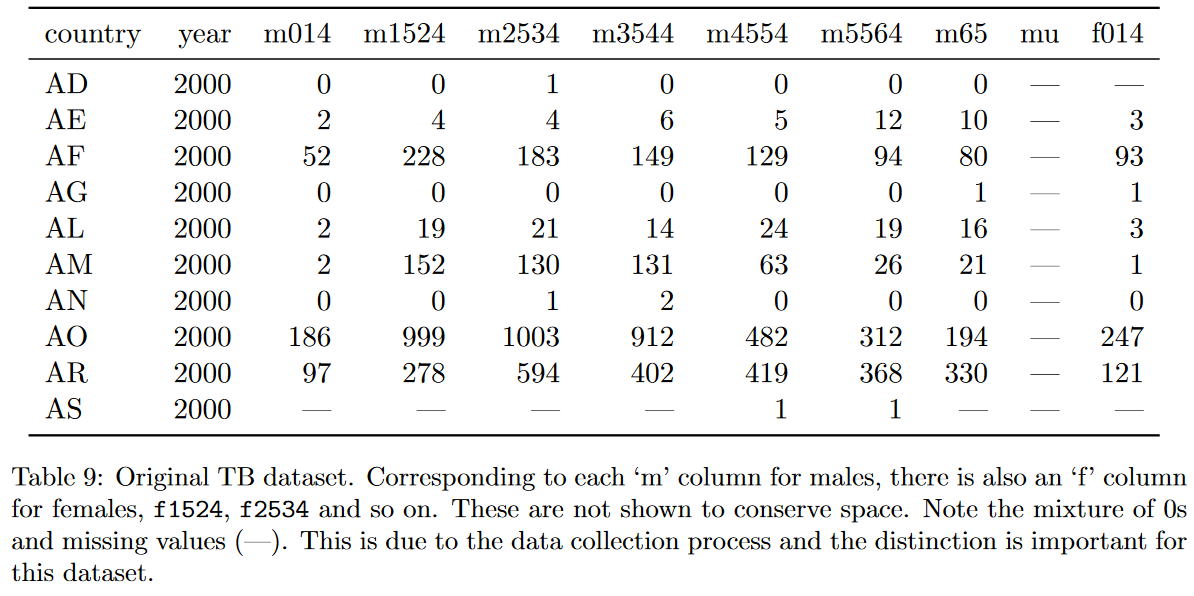
Figure 6.3: Table 9 from the “Tidy Data” paper, showing a subset of TB case counts. The columns are ‘country’, ‘year’, and demographic information combining gender and age group, e.g., male aged 0 to 14 as ‘m014’
Combining multiple bits of information in a column is fairly common in medical data sets. If we look at just the column names, we can see that we have a similar problem from the previous example (Section TODO). So we would fix that problem first (Panel A in Figure TODO). From there we can “split” the gender information from the “age” information to separate from one another and create separate columns (Panel B in Figure TODO).
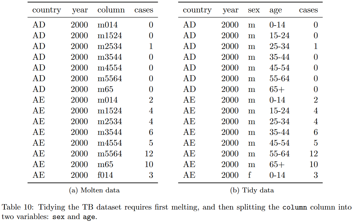
Figure 6.4: Table 10 from the “Tidy Data” paper
Let’s go through this example from the paper ourselves.
R
# read the tb dataset
tb <- read_csv("./data/tb_long.csv")
tb
# A tibble: 201 × 18
country year m014 m1524 m2534 m3544 m4554 m5564 m65 mu f014 f1524
<chr> <dbl> <dbl> <dbl> <dbl> <dbl> <dbl> <dbl> <dbl> <lgl> <dbl> <dbl>
1 AD 2000 0 0 1 0 0 0 0 NA NA NA
2 AE 2000 2 4 4 6 5 12 10 NA 3 16
3 AF 2000 52 228 183 149 129 94 80 NA 93 414
4 AG 2000 0 0 0 0 0 0 1 NA 1 1
5 AL 2000 2 19 21 14 24 19 16 NA 3 11
6 AM 2000 2 152 130 131 63 26 21 NA 1 24
7 AN 2000 0 0 1 2 0 0 0 NA 0 0
8 AO 2000 186 999 1003 912 482 312 194 NA 247 1142
9 AR 2000 97 278 594 402 419 368 330 NA 121 544
10 AS 2000 NA NA NA NA 1 1 NA NA NA NA
# … with 191 more rows, and 6 more variables: f2534 <dbl>, f3544 <dbl>,
# f4554 <dbl>, f5564 <dbl>, f65 <dbl>, fu <lgl>Python
tb = pd.read_csv("./data/tb_long.csv")
tb
country year m014 m1524 m2534 ... f3544 f4554 f5564 f65 fu
0 AD 2000 0.0 0.0 1.0 ... NaN NaN NaN NaN NaN
1 AE 2000 2.0 4.0 4.0 ... 3.0 0.0 0.0 4.0 NaN
2 AF 2000 52.0 228.0 183.0 ... 339.0 205.0 99.0 36.0 NaN
3 AG 2000 0.0 0.0 0.0 ... 0.0 0.0 0.0 0.0 NaN
4 AL 2000 2.0 19.0 21.0 ... 8.0 8.0 5.0 11.0 NaN
.. ... ... ... ... ... ... ... ... ... ... ..
196 YE 2000 110.0 789.0 689.0 ... 517.0 345.0 247.0 92.0 NaN
197 YU 2000 NaN NaN NaN ... NaN NaN NaN NaN NaN
198 ZA 2000 116.0 723.0 1999.0 ... 933.0 423.0 167.0 80.0 NaN
199 ZM 2000 349.0 2175.0 2610.0 ... 1305.0 186.0 112.0 75.0 NaN
200 ZW 2000 NaN NaN NaN ... NaN NaN NaN NaN NaN
[201 rows x 18 columns]R
Our first step is to make our data long using the pivot_longer function.
Here we are using a different method to select our columns using the starts_with selector.
You can also use the previous range selector as well.
tb_tidy <- tb %>%
  pivot_longer(starts_with(c('m', 'f')))
tb_tidy
# A tibble: 3,216 × 4
country year name value
<chr> <dbl> <chr> <dbl>
1 AD 2000 m014 0
2 AD 2000 m1524 0
3 AD 2000 m2534 1
4 AD 2000 m3544 0
5 AD 2000 m4554 0
6 AD 2000 m5564 0
7 AD 2000 m65 0
8 AD 2000 mu NA
9 AD 2000 f014 NA
10 AD 2000 f1524 NA
# … with 3,206 more rowsPython
tb_tidy = tb.melt(id_vars=["country", "year"])
tb_tidy
country year variable value
0 AD 2000 m014 0.0
1 AE 2000 m014 2.0
2 AF 2000 m014 52.0
3 AG 2000 m014 0.0
4 AL 2000 m014 2.0
... ... ... ... ...
3211 YE 2000 fu NaN
3212 YU 2000 fu NaN
3213 ZA 2000 fu NaN
3214 ZM 2000 fu NaN
3215 ZW 2000 fu NaN
[3216 rows x 4 columns]R
Now that we have the “long” dataset, we can use the separate function to separate out the information in that column.
tb_tidy <- tb_tidy %>%
  separate(name, into = c("sex", "age_group"), sep = 1)
tb_tidy
# A tibble: 3,216 × 5
country year sex age_group value
<chr> <dbl> <chr> <chr> <dbl>
1 AD 2000 m 014 0
2 AD 2000 m 1524 0
3 AD 2000 m 2534 1
4 AD 2000 m 3544 0
5 AD 2000 m 4554 0
6 AD 2000 m 5564 0
7 AD 2000 m 65 0
8 AD 2000 m u NA
9 AD 2000 f 014 NA
10 AD 2000 f 1524 NA
# … with 3,206 more rowsPython
tb_tidy["sex"] = tb_tidy["variable"].str.slice(start=0, stop=1) # can also do .str.get(0)
tb_tidy["age_group"] = tb_tidy["variable"].str.slice(start=1)
tb_tidy
country year variable value sex age_group
0 AD 2000 m014 0.0 m 014
1 AE 2000 m014 2.0 m 014
2 AF 2000 m014 52.0 m 014
3 AG 2000 m014 0.0 m 014
4 AL 2000 m014 2.0 m 014
... ... ... ... ... .. ...
3211 YE 2000 fu NaN f u
3212 YU 2000 fu NaN f u
3213 ZA 2000 fu NaN f u
3214 ZM 2000 fu NaN f u
3215 ZW 2000 fu NaN f u
[3216 rows x 6 columns]Technically the pivot_longer function provides the ability to do the pivot and separation in a single step,
but this way we see the parts broken down into separate components.
When curating your own data set, leave yourself a bread-trail to process your data later on.
6.6 Variables are stored in both rows and columns
The last common data problem we can have is having variables stored in both rows and columns. This problem isn’t usually noticeable at first glance, and is only realized as you start fixing problems one step at a time.
The first thing we’ll see is that we have the same columns as variables problem we’ve been having this entire time. So we can fix the variables being stored in the columns the same way as we have been doing.
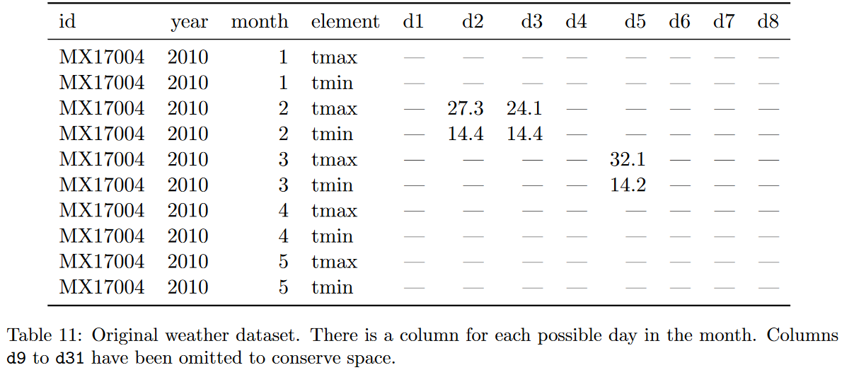
Figure 6.5: Table 11 from the “Tidy Data” paper
Only after we fix the column problem, do we see that somthing is a little off about our dataset. The weather information is usually report at the “day” level. That is, every observation is a day, and we should have a maximum and minimum temperature value for each day. However, in the initial “long” data set format, we see that the data is stored by date and element values.
Another symptom of data being stored in rows is a lot of repeated column values with only a few changes in cells between rows.
The way we fix the “variables stored in row” problem is to perform the “opposite” of the pivot_longer function we have been using.
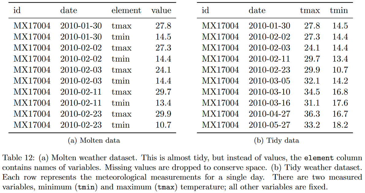
Figure 6.6: Table 12 from the “Tidy Data” paper
We can load up the CMS utilization dataset that gives us CMS utilization rates by state, demographics, year, and measurement.
R
cms <- read_csv("./data/cms_utilization.csv")
cms
# A tibble: 3,456 × 17
state state_fips variable sex age_group num_chronic `2007` `2008` `2009`
<chr> <chr> <chr> <chr> <chr> <chr> <dbl> <dbl> <dbl>
1 Alabama 01 Per Capi… males Less tha… 0 to 1 1594. 1640. 1680.
2 Alabama 01 Per Capi… males Less tha… 2 to 3 6269. 6484. 6339.
3 Alabama 01 Per Capi… males Less tha… 4 to 5 12902. 13400. 13713.
4 Alabama 01 Per Capi… males Less tha… 6+ 31169. 32837. 33190.
5 Alabama 01 Per Capi… males Less tha… 0 to 1 1745. 1794. 1829.
6 Alabama 01 Per Capi… males Less tha… 2 to 3 6752. 7035. 6816.
7 Alabama 01 Per Capi… males Less tha… 4 to 5 13796. 14385. 14596.
8 Alabama 01 Per Capi… males Less tha… 6+ 32779. 34641. 34879.
9 Alabama 01 ED Visit… males Less tha… 0 to 1 398. 410. 411.
10 Alabama 01 ED Visit… males Less tha… 2 to 3 865. 865. 852.
# … with 3,446 more rows, and 8 more variables: 2010 <dbl>, 2011 <dbl>,
# 2012 <dbl>, 2013 <dbl>, 2014 <dbl>, 2015 <dbl>, 2016 <dbl>, 2017 <dbl>Python
cms = pd.read_csv("./data/cms_utilization.csv")
cms
state state_fips variable sex \
0 Alabama 1.0 Per Capita Spending-Actual ($) males
1 Alabama 1.0 Per Capita Spending-Actual ($) males
2 Alabama 1.0 Per Capita Spending-Actual ($) males
3 Alabama 1.0 Per Capita Spending-Actual ($) males
4 Alabama 1.0 Per Capita Spending-Standardized ($) males
... ... ... ... ...
3451 Unknown NaN ED Visits per 1,000 Beneficiaries females
3452 Unknown NaN Hospital Readmissions-Percentage (%) females
3453 Unknown NaN Hospital Readmissions-Percentage (%) females
3454 Unknown NaN Hospital Readmissions-Percentage (%) females
3455 Unknown NaN Hospital Readmissions-Percentage (%) females
age_group ... 2013 2014 2015 \
0 Less than 65 Years ... 1729.1753 1791.3835 1868.3037
1 Less than 65 Years ... 5919.0137 6301.1517 6336.1253
2 Less than 65 Years ... 12513.1996 12466.4416 12095.8047
3 Less than 65 Years ... 32833.1685 32290.1432 31581.3385
4 Less than 65 Years ... 1891.0444 1914.9913 2029.6522
... ... ... ... ... ...
3451 65 Years and Over ... NaN NaN NaN
3452 65 Years and Over ... NaN NaN NaN
3453 65 Years and Over ... NaN NaN NaN
3454 65 Years and Over ... NaN NaN NaN
3455 65 Years and Over ... NaN NaN NaN
2016 2017
0 1735.7188 1835.0004
1 6470.7950 6126.4439
2 11441.0180 12181.1097
3 31392.0268 31770.9529
4 1909.2177 2003.7819
... ... ...
3451 NaN NaN
3452 NaN NaN
3453 NaN NaN
3454 NaN NaN
3455 NaN NaN
[3456 rows x 17 columns]We can make our data “long” just like before.
R
cms_long <- cms %>%
  pivot_longer(`2007`:last_col(), names_to = "year")
cms_long
# A tibble: 38,016 × 8
state state_fips variable sex age_group num_chronic year value
<chr> <chr> <chr> <chr> <chr> <chr> <chr> <dbl>
1 Alabama 01 Per Capita Spen… males Less than … 0 to 1 2007 1594.
2 Alabama 01 Per Capita Spen… males Less than … 0 to 1 2008 1640.
3 Alabama 01 Per Capita Spen… males Less than … 0 to 1 2009 1680.
4 Alabama 01 Per Capita Spen… males Less than … 0 to 1 2010 1599.
5 Alabama 01 Per Capita Spen… males Less than … 0 to 1 2011 1612.
6 Alabama 01 Per Capita Spen… males Less than … 0 to 1 2012 1695.
7 Alabama 01 Per Capita Spen… males Less than … 0 to 1 2013 1729.
8 Alabama 01 Per Capita Spen… males Less than … 0 to 1 2014 1791.
9 Alabama 01 Per Capita Spen… males Less than … 0 to 1 2015 1868.
10 Alabama 01 Per Capita Spen… males Less than … 0 to 1 2016 1736.
# … with 38,006 more rowsPython
cms.columnsIndex(['state', 'state_fips', 'variable', 'sex', 'age_group', 'num_chronic',
'2007', '2008', '2009', '2010', '2011', '2012', '2013', '2014', '2015',
'2016', '2017'],
dtype='object')cms_long = cms.melt(id_vars=['state', 'state_fips', 'variable', 'sex', 'age_group', 'num_chronic'],
var_name="year")
cms_long state state_fips variable sex \
0 Alabama 1.0 Per Capita Spending-Actual ($) males
1 Alabama 1.0 Per Capita Spending-Actual ($) males
2 Alabama 1.0 Per Capita Spending-Actual ($) males
3 Alabama 1.0 Per Capita Spending-Actual ($) males
4 Alabama 1.0 Per Capita Spending-Standardized ($) males
... ... ... ... ...
38011 Unknown NaN ED Visits per 1,000 Beneficiaries females
38012 Unknown NaN Hospital Readmissions-Percentage (%) females
38013 Unknown NaN Hospital Readmissions-Percentage (%) females
38014 Unknown NaN Hospital Readmissions-Percentage (%) females
38015 Unknown NaN Hospital Readmissions-Percentage (%) females
age_group num_chronic year value
0 Less than 65 Years 0 to 1 2007 1593.9423
1 Less than 65 Years 2 to 3 2007 6269.3549
2 Less than 65 Years 4 to 5 2007 12901.7265
3 Less than 65 Years 6+ 2007 31168.6543
4 Less than 65 Years 0 to 1 2007 1745.4352
... ... ... ... ...
38011 65 Years and Over 6+ 2017 NaN
38012 65 Years and Over 0 to 1 2017 NaN
38013 65 Years and Over 2 to 3 2017 NaN
38014 65 Years and Over 4 to 5 2017 NaN
38015 65 Years and Over 6+ 2017 NaN
[38016 rows x 8 columns]Now when we want to use the pivot_wider function, we want to specify the column we want to pivot.
During this process, every unique value in this column will become a separate column.
The next thing we need to provide is the column that will be used to fill in the body of the cells when the column is pivoted.
R
cms_tidy <- cms_long %>%
  pivot_wider(names_from = variable, values_from = value)
cms_tidy
# A tibble: 9,504 × 10
state state_fips sex age_group num_chronic year `Per Capita Spe…
<chr> <chr> <chr> <chr> <chr> <chr> <dbl>
1 Alabama 01 males Less than 65 Years 0 to 1 2007 1594.
2 Alabama 01 males Less than 65 Years 0 to 1 2008 1640.
3 Alabama 01 males Less than 65 Years 0 to 1 2009 1680.
4 Alabama 01 males Less than 65 Years 0 to 1 2010 1599.
5 Alabama 01 males Less than 65 Years 0 to 1 2011 1612.
6 Alabama 01 males Less than 65 Years 0 to 1 2012 1695.
7 Alabama 01 males Less than 65 Years 0 to 1 2013 1729.
8 Alabama 01 males Less than 65 Years 0 to 1 2014 1791.
9 Alabama 01 males Less than 65 Years 0 to 1 2015 1868.
10 Alabama 01 males Less than 65 Years 0 to 1 2016 1736.
# … with 9,494 more rows, and 3 more variables:
# Per Capita Spending-Standardized ($) <dbl>,
# ED Visits per 1,000 Beneficiaries <dbl>,
# Hospital Readmissions-Percentage (%) <dbl>Python
cms_long.columnsIndex(['state', 'state_fips', 'variable', 'sex', 'age_group', 'num_chronic',
'year', 'value'],
dtype='object')cms_tidy = cms_long.pivot(index=['state', 'state_fips', 'sex', 'age_group', 'num_chronic', 'year'],
columns="variable",
values="value")
cms_tidyvariable ED Visits per 1,000 Beneficiaries \
state state_fips sex age_group num_chronic year
Alabama 1.0 females 65 Years and Over 0 to 1 2007 133.2392
2008 132.5548
2009 126.6189
2010 130.7295
2011 123.7849
... ...
Wyoming 56.0 males Less than 65 Years 6+ 2013 3518.1058
2014 3466.8588
2015 3734.4111
2016 3806.8966
2017 3636.9427
variable Hospital Readmissions-Percentage (%) \
state state_fips sex age_group num_chronic year
Alabama 1.0 females 65 Years and Over 0 to 1 2007 5.24
2008 5.93
2009 5.36
2010 5.19
2011 5.16
... ...
Wyoming 56.0 males Less than 65 Years 6+ 2013 23.69
2014 21.56
2015 23.29
2016 27.26
2017 26.68
variable Per Capita Spending-Actual ($) \
state state_fips sex age_group num_chronic year
Alabama 1.0 females 65 Years and Over 0 to 1 2007 1802.9955
2008 1826.0823
2009 1860.5879
2010 1955.1089
2011 1890.8935
... ...
Wyoming 56.0 males Less than 65 Years 6+ 2013 38811.7588
2014 38674.4340
2015 41523.8245
2016 41411.0227
2017 42182.9795
variable Per Capita Spending-Standardized ($)
state state_fips sex age_group num_chronic year
Alabama 1.0 females 65 Years and Over 0 to 1 2007 1982.1296
2008 2007.3557
2009 2036.4565
2010 2101.6307
2011 2046.3090
... ...
Wyoming 56.0 males Less than 65 Years 6+ 2013 34426.4124
2014 35370.7925
2015 36567.3271
2016 36058.6849
2017 37148.7624
[9504 rows x 4 columns]cms_tidy = (cms_long
.pivot(index=['state', 'state_fips', 'sex', 'age_group', 'num_chronic', 'year'],
columns="variable",
values="value")
.reset_index()
)
cms_tidyvariable state state_fips sex age_group num_chronic year \
0 Alabama 1.0 females 65 Years and Over 0 to 1 2007
1 Alabama 1.0 females 65 Years and Over 0 to 1 2008
2 Alabama 1.0 females 65 Years and Over 0 to 1 2009
3 Alabama 1.0 females 65 Years and Over 0 to 1 2010
4 Alabama 1.0 females 65 Years and Over 0 to 1 2011
... ... ... ... ... ... ...
9499 Wyoming 56.0 males Less than 65 Years 6+ 2013
9500 Wyoming 56.0 males Less than 65 Years 6+ 2014
9501 Wyoming 56.0 males Less than 65 Years 6+ 2015
9502 Wyoming 56.0 males Less than 65 Years 6+ 2016
9503 Wyoming 56.0 males Less than 65 Years 6+ 2017
variable ED Visits per 1,000 Beneficiaries \
0 133.2392
1 132.5548
2 126.6189
3 130.7295
4 123.7849
... ...
9499 3518.1058
9500 3466.8588
9501 3734.4111
9502 3806.8966
9503 3636.9427
variable Hospital Readmissions-Percentage (%) \
0 5.24
1 5.93
2 5.36
3 5.19
4 5.16
... ...
9499 23.69
9500 21.56
9501 23.29
9502 27.26
9503 26.68
variable Per Capita Spending-Actual ($) Per Capita Spending-Standardized ($)
0 1802.9955 1982.1296
1 1826.0823 2007.3557
2 1860.5879 2036.4565
3 1955.1089 2101.6307
4 1890.8935 2046.3090
... ... ...
9499 38811.7588 34426.4124
9500 38674.4340 35370.7925
9501 41523.8245 36567.3271
9502 41411.0227 36058.6849
9503 42182.9795 37148.7624
[9504 rows x 10 columns]6.7 Summary
Tidy data is a common “format” that lets data be interoperable with all of the analytics tools. Once your data is “tidy”, you can easily create summary statistics, plots, and fit models.
 blog [*Tidy Data for reproducibility, efficiency, and collaboration*](https://www.openscapes.org/blog/2020/10/12/tidy-data/) by Julia Lowndes and Allison Horst](https://github.com/allisonhorst/stats-illustrations/raw/master/rstats-artwork/tidydata_5.jpg)
Figure 6.7: Illustrations from the Openscapes blog Tidy Data for reproducibility, efficiency, and collaboration by Julia Lowndes and Allison Horst
Most of your data processing phase will be spent wrangling data into a tidy format.
 blog [*Tidy Data for reproducibility, efficiency, and collaboration*](https://www.openscapes.org/blog/2020/10/12/tidy-data/) by Julia Lowndes and Allison Horst](https://github.com/allisonhorst/stats-illustrations/raw/master/rstats-artwork/tidydata_6.jpg)
Figure 6.8: Illustrations from the Openscapes blog Tidy Data for reproducibility, efficiency, and collaboration by Julia Lowndes and Allison Horst
But once it’s there, you can easily create other data products from them, including non-tidy data for presentations.
 blog [*Tidy Data for reproducibility, efficiency, and collaboration*](https://www.openscapes.org/blog/2020/10/12/tidy-data/) by Julia Lowndes and Allison Horst](https://github.com/allisonhorst/stats-illustrations/raw/master/rstats-artwork/tidydata_7.jpg)
Figure 6.9: Illustrations from the Openscapes blog Tidy Data for reproducibility, efficiency, and collaboration by Julia Lowndes and Allison Horst
6.8 Additional Resources
- Tidy data paper: https://vita.had.co.nz/papers/tidy-data.html
- More code heavy R documentation on tidy data: https://cran.r-project.org/web/packages/tidyr/vignettes/tidy-data.html
- r4ds Tidy Data Chapter: https://r4ds.had.co.nz/tidy-data.html