Chapter 8 Analysis Intro
An introduction to analysis.
Learning how to read output.
8.1 Logistic Regression
library(medicaldata)
library(tidyverse)
blood <- blood_storageVariable of interest: Recurrence. It is a binary variable that only has 2 possible values.
blood %>%
  group_by(Recurrence) %>%
  summarize(count = n())
# A tibble: 2 × 2
Recurrence count
<dbl> <int>
1 0 262
2 1 54Logistic regression is linear regression using the logit function as a transformation.
\(\text{logit}(p) = log(\frac{p}{1 - p})\)
Since it is a form of a linear regression, it is known as a generalized linear regression method (GLM).
We can use the glm function in R.
8.1.1 Model 1
mod1 <- glm(Recurrence ~ Age, data = blood, family = "binomial")mod1
Call:  glm(formula = Recurrence ~ Age, family = "binomial", data = blood)

Coefficients:
(Intercept)          Age
   -2.51068      0.01516

Degrees of Freedom: 315 Total (i.e. Null);  314 Residual
Null Deviance:      289
Residual Deviance: 288.5 AIC: 292.5summary(mod1)
Call:
glm(formula = Recurrence ~ Age, family = "binomial", data = blood)

Deviance Residuals:
    Min       1Q   Median       3Q      Max
-0.6806  -0.6263  -0.6050  -0.5702   2.0050

Coefficients:
            Estimate Std. Error z value Pr(>|z|)
(Intercept) -2.51068    1.30197  -1.928   0.0538 .
Age          0.01516    0.02097   0.723   0.4696
---
Signif. codes:  0 '***' 0.001 '**' 0.01 '*' 0.05 '.' 0.1 ' ' 1

(Dispersion parameter for binomial family taken to be 1)

    Null deviance: 289.01  on 315  degrees of freedom
Residual deviance: 288.48  on 314  degrees of freedom
AIC: 292.48

Number of Fisher Scoring iterations: 4library(broom)res1 <- tidy(mod1)
res1# A tibble: 2 × 5
term estimate std.error statistic p.value
<chr> <dbl> <dbl> <dbl> <dbl>
1 (Intercept) -2.51 1.30 -1.93 0.0538
2 Age 0.0152 0.0210 0.723 0.470 Whatever we do after fitting the model, we have to undo the logit function for interpretation. Otherwise all the values have to be interpreted as “log-odds” which is not intutitive.
However, “odds” is intuitive, so we only really need to undo the “log”. We do this by exponentiation.
res1 %>%
  mutate(odds = exp(estimate))
# A tibble: 2 × 6
term estimate std.error statistic p.value odds
<chr> <dbl> <dbl> <dbl> <dbl> <dbl>
1 (Intercept) -2.51 1.30 -1.93 0.0538 0.0812
2 Age 0.0152 0.0210 0.723 0.470 1.02 For every 1 unit increase in Age, the odds of going from 0 to 1 in our response increases by 1.02 times.
That is, the odds of earlier biochemical recurrence of prostate cancer after prostatectomy increases by 1.02 times for every unit increase in age.
8.1.2 Model 2
PVol: Prostate volumn in grams (g)PreopPSA: Preoperative prostate specification antigen (PSA) in ng/mL
mod2 <- glm(Recurrence ~ Age + PVol + PreopPSA, data = blood, family = "binomial")
summary(mod2)
Call:
glm(formula = Recurrence ~ Age + PVol + PreopPSA, family = "binomial",
    data = blood)

Deviance Residuals:
    Min       1Q   Median       3Q      Max
-1.6531  -0.5795  -0.5174  -0.4541   2.1774

Coefficients:
             Estimate Std. Error z value Pr(>|z|)
(Intercept) -3.756396   1.438716  -2.611  0.00903 **
Age          0.028142   0.023570   1.194  0.23249
PVol        -0.007971   0.005828  -1.368  0.17140
PreopPSA     0.095164   0.023055   4.128 3.66e-05 ***
---
Signif. codes:  0 '***' 0.001 '**' 0.01 '*' 0.05 '.' 0.1 ' ' 1

(Dispersion parameter for binomial family taken to be 1)

    Null deviance: 275.38  on 304  degrees of freedom
Residual deviance: 257.04  on 301  degrees of freedom
  (11 observations deleted due to missingness)
AIC: 265.04

Number of Fisher Scoring iterations: 4
mod2 %>%
tidy() %>%
mutate(odds = exp(estimate))# A tibble: 4 × 6
term estimate std.error statistic p.value odds
<chr> <dbl> <dbl> <dbl> <dbl> <dbl>
1 (Intercept) -3.76 1.44 -2.61 0.00903 0.0234
2 Age 0.0281 0.0236 1.19 0.232 1.03
3 PVol -0.00797 0.00583 -1.37 0.171 0.992
4 PreopPSA 0.0952 0.0231 4.13 0.0000366 1.10 That is, the odds of earlier biochemical recurrence of prostate cancer after prostatectomy increases by 1.10 times for every unit increase in PreopPSA, all else equal.
ggplot(blood, aes(x = PreopPSA)) +
  geom_histogram()
`stat_bin()` using `bins = 30`. Pick better value with `binwidth`.Warning: Removed 3 rows containing non-finite values (stat_bin).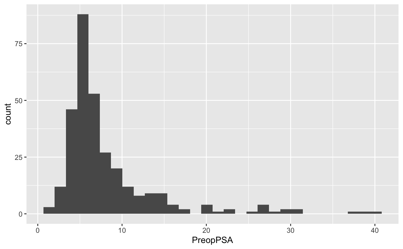
8.1.3 Model 3
TVolTumor volume- 1 = Low
- 2 = Medium
- 3 = Extensive
mod3 <- glm(Recurrence ~ Age + PVol + PreopPSA + TVol, data = blood, family = "binomial")
summary(mod3)
Call:
glm(formula = Recurrence ~ Age + PVol + PreopPSA + TVol, family = "binomial",
    data = blood)

Deviance Residuals:
    Min       1Q   Median       3Q      Max
-1.4786  -0.5536  -0.4379  -0.2406   2.4177

Coefficients:
             Estimate Std. Error z value Pr(>|z|)
(Intercept) -6.736029   1.734337  -3.884 0.000103 ***
Age          0.028789   0.024511   1.175 0.240180
PVol        -0.001004   0.006215  -0.162 0.871697
PreopPSA     0.057670   0.024212   2.382 0.017224 *
TVol         1.231067   0.298191   4.128 3.65e-05 ***
---
Signif. codes:  0 '***' 0.001 '**' 0.01 '*' 0.05 '.' 0.1 ' ' 1

(Dispersion parameter for binomial family taken to be 1)

    Null deviance: 267.09  on 299  degrees of freedom
Residual deviance: 230.30  on 295  degrees of freedom
  (16 observations deleted due to missingness)
AIC: 240.3

Number of Fisher Scoring iterations: 5
How do you interpret “one unit increase in Tvol (Tumor volume), it is a categorical variable.
It’s”ordinal” so you may be able to get away with the interpretation,
but there is no way the value can be 1.5.
How do we handle categorical variables? We use as.factor.
mod3_factor <- glm(Recurrence ~ Age + PVol + PreopPSA + as.factor(TVol), data = blood, family = "binomial")
summary(mod3_factor)
Call:
glm(formula = Recurrence ~ Age + PVol + PreopPSA + as.factor(TVol),
    family = "binomial", data = blood)

Deviance Residuals:
    Min       1Q   Median       3Q      Max
-1.4726  -0.5886  -0.4641  -0.1714   2.6700

Coefficients:
                   Estimate Std. Error z value Pr(>|z|)
(Intercept)      -6.140e+00  1.819e+00  -3.375 0.000738 ***
Age               2.654e-02  2.453e-02   1.082 0.279289
PVol             -9.982e-06  6.494e-03  -0.002 0.998773
PreopPSA          5.860e-02  2.419e-02   2.422 0.015441 *
as.factor(TVol)2  2.073e+00  1.061e+00   1.954 0.050724 .
as.factor(TVol)3  3.120e+00  1.064e+00   2.931 0.003379 **
---
Signif. codes:  0 '***' 0.001 '**' 0.01 '*' 0.05 '.' 0.1 ' ' 1

(Dispersion parameter for binomial family taken to be 1)

    Null deviance: 267.09  on 299  degrees of freedom
Residual deviance: 229.39  on 294  degrees of freedom
  (16 observations deleted due to missingness)
AIC: 241.39

Number of Fisher Scoring iterations: 6
Notice one of the factors was dropped, this is called the reference variable. We converted our categorical variable into a set of dummy variables (aka one-hot encoding).
model.matrix(mod3_factor) %>%
  head()
(Intercept) Age PVol PreopPSA as.factor(TVol)2 as.factor(TVol)3
1 1 72.1 54.0 14.08 0 1
2 1 73.6 43.2 10.50 0 1
3 1 67.5 102.7 6.98 0 0
4 1 65.8 46.0 4.40 0 0
5 1 63.2 60.0 21.40 1 0
6 1 65.4 45.9 5.10 1 0mod3_factor %>%
tidy() %>%
mutate(odds = exp(estimate))# A tibble: 6 × 6
term estimate std.error statistic p.value odds
<chr> <dbl> <dbl> <dbl> <dbl> <dbl>
1 (Intercept) -6.14 1.82 -3.38 0.000738 0.00216
2 Age 0.0265 0.0245 1.08 0.279 1.03
3 PVol -0.00000998 0.00649 -0.00154 0.999 1.00
4 PreopPSA 0.0586 0.0242 2.42 0.0154 1.06
5 as.factor(TVol)2 2.07 1.06 1.95 0.0507 7.95
6 as.factor(TVol)3 3.12 1.06 2.93 0.00338 22.6 That is, the odds of earlier biochemical recurrence of prostate cancer after prostatectomy increases by 22.6 times when the patient has a TVol (tumor volume) of “Extensive” when compared to “Low”.
All else equal.
# save the above table
mod_3_or_table <- mod3_factor %>%
  tidy() %>%
  mutate(odds = exp(estimate))
#plot the coefficients
ggplot(data = mod_3_or_table, aes(x = term, y = odds)) +
geom_point() +
geom_hline(yintercept = 1) +
coord_flip()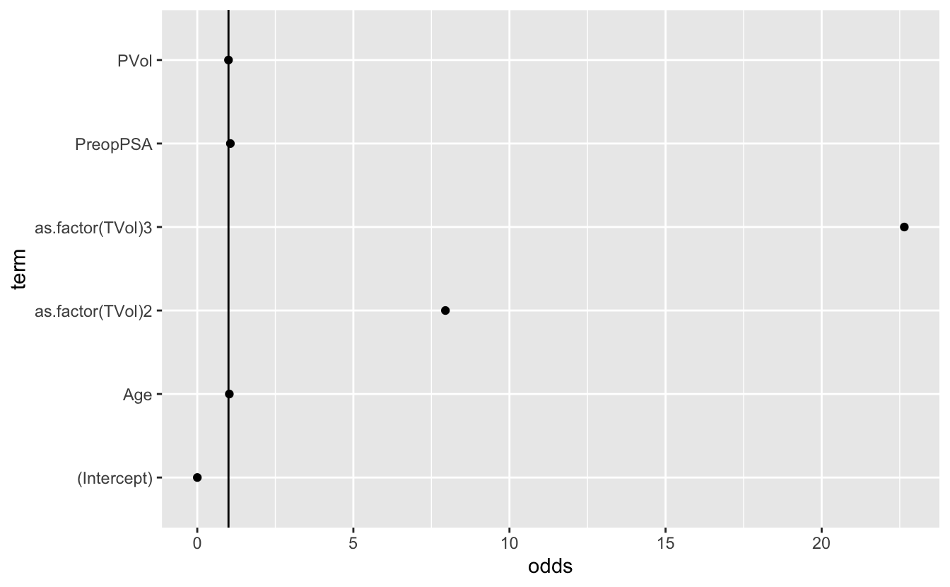
# add in confidence intervals
ci <- confint(mod3_factor, level = 0.95) %>%
  as.data.frame()
Waiting for profiling to be done...ci 2.5 % 97.5 %
(Intercept) -10.11472570 -2.80156779
Age -0.02079990 0.07580323
PVol -0.01354803 0.01278682
PreopPSA 0.01149335 0.10753271
as.factor(TVol)2 0.40898977 4.99920179
as.factor(TVol)3 1.44958506 6.05039015exp(ci) 2.5 % 97.5 %
(Intercept) 4.047906e-05 0.0607148
Age 9.794149e-01 1.0787503
PVol 9.865433e-01 1.0128689
PreopPSA 1.011560e+00 1.1135273
as.factor(TVol)2 1.505296e+00 148.2947414
as.factor(TVol)3 4.261346e+00 424.2785317mod3_or_ci <- mod_3_or_table %>%
mutate(ci_lower = exp(estimate - (1.96 * std.error)),
ci_upper = exp(estimate + (1.96 * std.error)))ggplot(mod3_or_ci) +
geom_point(aes(x = term, y = odds)) +
geom_errorbar(aes(x = term, ymin = ci_lower, ymax = ci_upper)) +
coord_flip()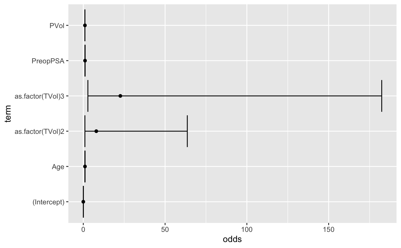
\(y = mx + b\)
\(y = \text{intercept} + \beta_1x_1 + \beta_2x_2 + \beta_3x_3 + \beta_4x_4 + e + \beta_5x_5 + e\)
- \(\beta_1\):
Age - \(\beta_2\):
PVol - \(\beta_3\):
PreopPSA - \(\beta_4\):
TVol2 - \(\beta_5\):
TVol3
\(\hat{y} = \text{intercept} + \beta_1x_1 + \beta_2x_2 + \beta_3x_3 + \beta_4x_4 + \beta_5x_5\)
\(log(\frac{p}{1 - p}) = \text{intercept} + \beta_1x_1 + \beta_2x_2 + \beta_3x_3 + \beta_4x_4 + \beta_5x_5)\) \(\frac{p}{1 - p} = odds = e^{(\text{intercept} + \beta_1x_1 + \beta_2x_2 + \beta_3x_3 + \beta_4x_4 + \beta_5x_5)}\)
\(\beta = log(OR) \leftrightarrow e^{\beta} = OR\)
- Load the cytomegalovirus dataset from the
medicaldatalibrary, assign it to the variablecmv
library(tidyverse)
library(medicaldata)
____- Fit a model using the
cmvdataframe, and thecmvvariable as the reponse variable. Save the model to the variable,mod
mod <- glm(____, data = ____, family = "binomial")- Use the
summaryfunction to look at the model output
ggplot(____, aes(as.factor(____))) +
geom_bar(aes(fill = as.factor(____)))- Use the
tidyfunction from thebroompackage to get just the coefficients table. Save this table to the variablebetas
library(broom)
____ <- ____(____)- Convert the
estimatecolumn into anorcolumn using themutatefunction and exponentiating the column values with theexpfunction.
betas %>%
____(____ = ____(____))- Interpret one of your ORs
library(medicaldata)
cmv <- cytomegalovirus

mod <- glm(cmv ~ as.factor(diagnosis) + time.to.transplant + as.factor(recipient.cmv) + as.factor(donor.cmv),
           data = cmv,
           family = "binomial")

summary(mod)
Call:
glm(formula = cmv ~ as.factor(diagnosis) + time.to.transplant +
    as.factor(recipient.cmv) + as.factor(donor.cmv), family = "binomial",
    data = cmv)

Deviance Residuals:
    Min       1Q   Median       3Q      Max
-1.6885  -0.8056  -0.2249   0.8962   2.6195

Coefficients:
                                                   Estimate Std. Error z value
(Intercept)                                      -2.114e+01  3.956e+03  -0.005
as.factor(diagnosis)acute myeloid leukemia        1.745e+01  3.956e+03   0.004
as.factor(diagnosis)aplastic anemia               7.054e-03  5.595e+03   0.000
as.factor(diagnosis)chronic lymphocytic leukemia  1.984e+01  3.956e+03   0.005
as.factor(diagnosis)chronic myeloid leukemia      1.819e+01  3.956e+03   0.005
as.factor(diagnosis)congenital anemia            -9.548e-03  5.595e+03   0.000
as.factor(diagnosis)Hodgkin lymphoma              1.907e+01  3.956e+03   0.005
as.factor(diagnosis)multiple myelomas             2.019e+01  3.956e+03   0.005
as.factor(diagnosis)myelodysplastic syndrome      1.827e+01  3.956e+03   0.005
as.factor(diagnosis)myelofibrosis                 1.935e+01  3.956e+03   0.005
as.factor(diagnosis)myeloproliferative disorder   3.442e+00  5.595e+03   0.001
as.factor(diagnosis)non-Hodgkin lymphoma          1.772e+01  3.956e+03   0.004
as.factor(diagnosis)renal cell carcinoma          1.902e+01  3.956e+03   0.005
time.to.transplant                                7.379e-04  1.117e-02   0.066
as.factor(recipient.cmv)1                         2.433e+00  8.410e-01   2.893
as.factor(donor.cmv)1                             1.129e+00  7.429e-01   1.520
                                                 Pr(>|z|)
(Intercept)                                       0.99574
as.factor(diagnosis)acute myeloid leukemia        0.99648
as.factor(diagnosis)aplastic anemia               1.00000
as.factor(diagnosis)chronic lymphocytic leukemia  0.99600
as.factor(diagnosis)chronic myeloid leukemia      0.99633
as.factor(diagnosis)congenital anemia             1.00000
as.factor(diagnosis)Hodgkin lymphoma              0.99615
as.factor(diagnosis)multiple myelomas             0.99593
as.factor(diagnosis)myelodysplastic syndrome      0.99632
as.factor(diagnosis)myelofibrosis                 0.99610
as.factor(diagnosis)myeloproliferative disorder   0.99951
as.factor(diagnosis)non-Hodgkin lymphoma          0.99643
as.factor(diagnosis)renal cell carcinoma          0.99616
time.to.transplant                                0.94734
as.factor(recipient.cmv)1                         0.00382 **
as.factor(donor.cmv)1                             0.12857
---
Signif. codes:  0 '***' 0.001 '**' 0.01 '*' 0.05 '.' 0.1 ' ' 1

(Dispersion parameter for binomial family taken to be 1)

    Null deviance: 85.406  on 62  degrees of freedom
Residual deviance: 59.430  on 47  degrees of freedom
  (1 observation deleted due to missingness)
AIC: 91.43

Number of Fisher Scoring iterations: 16library(broom)
betas <- mod %>%
tidy()
betas# A tibble: 16 × 5
term estimate std.error statistic p.value
<chr> <dbl> <dbl> <dbl> <dbl>
1 (Intercept) -2.11e+1 3956. -5.34e-3 0.996
2 as.factor(diagnosis)acute myeloid leu… 1.74e+1 3956. 4.41e-3 0.996
3 as.factor(diagnosis)aplastic anemia 7.05e-3 5595. 1.26e-6 1.00
4 as.factor(diagnosis)chronic lymphocyt… 1.98e+1 3956. 5.02e-3 0.996
5 as.factor(diagnosis)chronic myeloid l… 1.82e+1 3956. 4.60e-3 0.996
6 as.factor(diagnosis)congenital anemia -9.55e-3 5595. -1.71e-6 1.00
7 as.factor(diagnosis)Hodgkin lymphoma 1.91e+1 3956. 4.82e-3 0.996
8 as.factor(diagnosis)multiple myelomas 2.02e+1 3956. 5.10e-3 0.996
9 as.factor(diagnosis)myelodysplastic s… 1.83e+1 3956. 4.62e-3 0.996
10 as.factor(diagnosis)myelofibrosis 1.94e+1 3956. 4.89e-3 0.996
11 as.factor(diagnosis)myeloproliferativ… 3.44e+0 5595. 6.15e-4 1.00
12 as.factor(diagnosis)non-Hodgkin lymph… 1.77e+1 3956. 4.48e-3 0.996
13 as.factor(diagnosis)renal cell carcin… 1.90e+1 3956. 4.81e-3 0.996
14 time.to.transplant 7.38e-4 0.0112 6.60e-2 0.947
15 as.factor(recipient.cmv)1 2.43e+0 0.841 2.89e+0 0.00382
16 as.factor(donor.cmv)1 1.13e+0 0.743 1.52e+0 0.129 betas %>%
mutate(or = exp(estimate))# A tibble: 16 × 6
term estimate std.error statistic p.value or
<chr> <dbl> <dbl> <dbl> <dbl> <dbl>
1 (Intercept) -2.11e+1 3956. -5.34e-3 0.996 6.62e-10
2 as.factor(diagnosis)acute my… 1.74e+1 3956. 4.41e-3 0.996 3.79e+ 7
3 as.factor(diagnosis)aplastic… 7.05e-3 5595. 1.26e-6 1.00 1.01e+ 0
4 as.factor(diagnosis)chronic … 1.98e+1 3956. 5.02e-3 0.996 4.14e+ 8
5 as.factor(diagnosis)chronic … 1.82e+1 3956. 4.60e-3 0.996 7.92e+ 7
6 as.factor(diagnosis)congenit… -9.55e-3 5595. -1.71e-6 1.00 9.90e- 1
7 as.factor(diagnosis)Hodgkin … 1.91e+1 3956. 4.82e-3 0.996 1.92e+ 8
8 as.factor(diagnosis)multiple… 2.02e+1 3956. 5.10e-3 0.996 5.88e+ 8
9 as.factor(diagnosis)myelodys… 1.83e+1 3956. 4.62e-3 0.996 8.61e+ 7
10 as.factor(diagnosis)myelofib… 1.94e+1 3956. 4.89e-3 0.996 2.53e+ 8
11 as.factor(diagnosis)myelopro… 3.44e+0 5595. 6.15e-4 1.00 3.13e+ 1
12 as.factor(diagnosis)non-Hodg… 1.77e+1 3956. 4.48e-3 0.996 4.99e+ 7
13 as.factor(diagnosis)renal ce… 1.90e+1 3956. 4.81e-3 0.996 1.82e+ 8
14 time.to.transplant 7.38e-4 0.0112 6.60e-2 0.947 1.00e+ 0
15 as.factor(recipient.cmv)1 2.43e+0 0.841 2.89e+0 0.00382 1.14e+ 1
16 as.factor(donor.cmv)1 1.13e+0 0.743 1.52e+0 0.129 3.09e+ 0